
Street-level traffic monitoring is a siting problem before it is a sensor problem
A useful network does not simply place more instruments along busy roads. It gives each monitoring point a defined role, keeps comparable sites genuinely comparable, and records enough context to explain why concentrations differ between places and times.
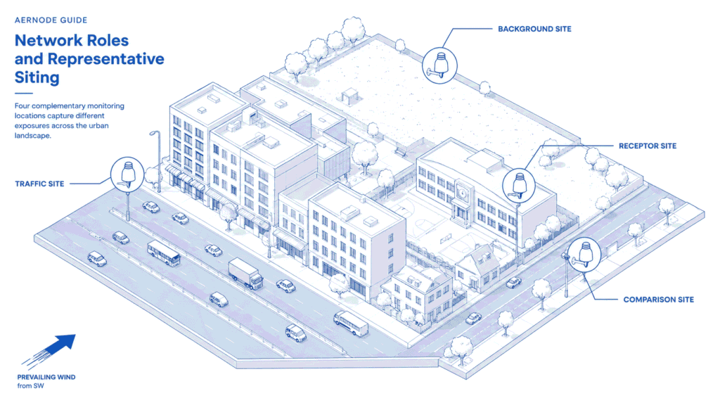
For a municipality, consultant or researcher, the practical question is usually not “where can a monitor be mounted?” but “what should this point represent?” A roadside hotspot, an urban-background location, a sensitive receptor and a corridor-comparison site answer different questions. If those roles are mixed together, a network can generate large data volumes without producing a defensible interpretation.
This Guide focuses on supplementary, continuous street-level networks used to characterize local traffic-related patterns and support investigation, planning or research. It does not replace formal ambient-air assessment. In Europe, Directive (EU) 2024/2881 sets specific requirements for sampling-point representativeness and siting when measurements are used within the statutory assessment framework. Those requirements provide an important reference, but they should not be treated as a universal mounting specification for every sensor project.
Start with the monitoring question, then define the site contrast
A street-level network becomes easier to design when the decision question is translated into a planned contrast between locations. The contrast is what makes the data interpretable.
| Monitoring question | Useful site contrast | What the comparison can support |
|---|---|---|
| Where are traffic-influenced concentrations highest? | Traffic-influenced roadside sites + nearby background | Screening of local spatial differences and candidate hotspots. |
| How do two corridors differ? | Comparable roadside sites on each corridor + common background context | Comparison while controlling, as far as practical, for siting and meteorological differences. |
| What conditions occur at a sensitive receptor? | Receptor site + nearest relevant traffic site + background | Understanding whether the receptor behaves more like the traffic corridor or the wider urban environment. |
| Did conditions change around a mobility intervention? | Stable before/after sites + a suitable comparison location | Evidence on temporal change; stronger interpretation when traffic and meteorology are also recorded. |
The number of nodes should follow the number of distinct environments that must be represented. Adding several instruments to effectively the same microenvironment may improve redundancy, but it does not automatically improve spatial understanding.
Build the network around distinct site roles
Roadside or traffic-influenced site
A roadside site is intentionally exposed to the influence of a defined traffic corridor. Select it because it represents a specific road type, traffic condition or street geometry – not simply because traffic is visible. Record traffic volume where available, lane arrangement, bus or freight activity, congestion patterns, road grade, nearby junctions, parking or loading activity, and the distance and orientation of the inlet relative to the carriageway.
Urban-background or neighbourhood comparison site
A background point provides context for interpreting whether a roadside location is elevated relative to the wider urban signal. The EU Directive describes urban-background sampling as being influenced by the integrated contribution from relevant sources rather than dominated by one source. For a supplementary network, the same principle is useful: choose a location that represents the broader area you intend to compare against, rather than a quiet corner with its own unusual microenvironment.
Sensitive-receptor or place-of-interest site
Schools, residential streets, hospitals, public spaces and other receptor locations can be useful when the project question is about conditions where people spend time. A receptor point should not be interpreted in isolation. Pairing it with traffic-influenced and background context helps determine whether the receptor pattern is more consistent with the local traffic environment or with wider urban and meteorological variation.
Replication across different street types
One roadside site cannot represent every road. Street canyons, open boulevards, elevated roads, bus corridors and freight routes can behave differently even at similar traffic counts. If the project must compare these environments, treat them as separate site classes and replicate the design rather than assuming one “traffic station” has a fixed coverage radius.
Choose pollutants and context variables to match the question
A traffic monitoring network should not use the largest available sensor package by default. Select parameters because they add information to the decision. For many street-level projects, NO2 and particulate matter provide a practical core, while other parameters add context for specific questions.
| Parameter | What it can add | Interpretation caution |
|---|---|---|
| NO2 | A strong traffic-relevant combustion indicator in many urban settings; useful for roadside-to-background contrast. | Not source-exclusive. Other combustion sources and atmospheric chemistry can affect concentrations. |
| PM2.5 / PM10 | Continuous information on fine and coarse particulate conditions around roads and neighbourhoods. | PM has regional and local contributions; traffic-related PM includes exhaust and non-exhaust sources, and optical measurements require sensor-specific QA. |
| CO | Additional combustion context in selected traffic environments. | Often a secondary parameter rather than the main network-design driver; usefulness depends on local levels and study objectives. |
| O3 | Useful wider urban photochemical context when the project needs it. | Ozone is secondary and should not be read as a simple direct traffic tracer; local NOx chemistry and regional background matter. |
| Meteorology | Wind speed/direction, temperature, humidity and pressure help explain transport, dispersion and sensor response. | Local wind around buildings may differ from a distant weather station; document where meteorological data come from. |
When NO2 is enough — and when NO / NOx adds value
For many municipal and street-level objectives, NO2 is the appropriate primary nitrogen-oxide parameter. It directly supports roadside-to-background comparison, local spatial screening, corridor and hotspot comparison, sensitive-receptor context and exposure-oriented urban monitoring, and it is the nitrogen-oxide pollutant with direct health-based ambient-air limit values in Directive (EU) 2024/2881. NO2 is sufficient when it already answers the monitoring question; adding NO does not automatically make a network better.
Adding NO becomes useful when the project needs a more detailed view of source-proximate combustion and nitrogen-oxide chemistry. Vehicle-related NOx contains both NO and NO2; U.S. EPA near-road technical guidance notes that a substantial part of fresh road-traffic NOx can be emitted as NO, while NO2 also occurs directly and the balance changes after emission as NO is oxidized, including through reaction with ozone. Measuring NO alongside NO2 can therefore reveal behaviour that NO2 alone does not fully resolve, without making NO a traffic-exclusive source marker or a source-attribution tool.
That second-level view can be useful at junctions and stop-start queues, in street canyons or other highly source-proximate locations, when comparing corridors with different fleet mix or operating conditions (including bus or freight corridors), or in detailed mobility-intervention, research or modelling work where NO / NO2 partitioning is itself relevant. O3 can add useful context when the project explicitly needs to interpret near-road NO / NO2 chemistry, but it is not a default requirement for every traffic network.
When NO and NO2 are measured separately, the channels can also support derived NOx analysis where appropriate. Do not create NOx by casually adding separately reported NO and NO2 mass concentrations without accounting for the unit convention: under the EU Directive, oxides of nitrogen are defined from the sum of the NO and NO2 volume mixing ratios and expressed as NO2-equivalent mass concentration. NOx is useful as a combustion-related parameter, but it is not traffic-exclusive and should not replace NO2 as the primary health-based metric for routine municipal monitoring.
For routine urban screening or exposure-oriented monitoring, NO2 may already answer the project question. Adding NO is most valuable when fresh combustion dynamics, NO / NO2 partitioning, derived NOx or more detailed source-proximate or intervention analysis are part of what the network needs to investigate.
Particulate monitoring also needs a clear measurement-method statement. A compact optical PM monitor can provide high-frequency spatial coverage, but it does not become a gravimetric reference method by reporting PM2.5 or PM10. See OPC and gravimetric PM measurement for the measurement-principle and data-quality distinction.
Traffic-related particulate matter is not only an exhaust question. The EMEP/EEA road-transport inventory guidance identifies tyre wear, brake wear and road-surface wear as non-exhaust particulate sources, so a roadside PM increase should not automatically be interpreted as a tailpipe signal. Where mechanically generated road dust or wear is part of the monitoring objective, coarse-particle monitoring can add useful context without uniquely identifying the source.
Specialist traffic-pollution studies may also use black carbon, ultrafine-particle number or chemical composition to answer narrower source or exposure questions. Those measurements require dedicated instrumentation and sit outside the standard measurement stack covered by this Guide. The network design principle remains the same: add a parameter only when it supports a defined question.
Street geometry can change what a roadside node sees
Traffic volume matters, but concentration at the inlet is also shaped by dispersion. The EU Directive explicitly requires road-traffic sampling locations to consider traffic volume, local dispersion conditions and spatial land use, including street canyons. The same variables are central to practical supplementary network design.
U.S.-specific EPA near-road NO2 technical guidance uses a similar site-selection logic: traffic volume, fleet mix, roadway design, congestion, terrain/topography and meteorology all affect where a near-road monitor is likely to capture the intended condition. These are transferable technical considerations, not European legal requirements.
Street canyons and building lines
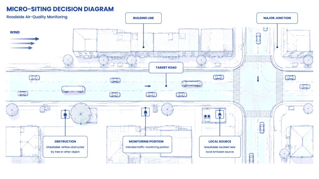
Continuous building facades can restrict dispersion and create large cross-street differences that vary with wind direction. If one node sits in a canyon while another is on an open boulevard, the comparison mixes traffic effects with urban-form effects. Either standardize the geometry or make the difference part of the study design and analysis.
Junctions, queues and stop-start activity
Intersections can create a microenvironment that differs from the rest of a road because traffic flow, acceleration and queuing change there. If the objective is to represent the wider road segment, avoid allowing a single junction to dominate the sample. If the objective is specifically to investigate junction conditions, treat it as a separate site class.
Barriers, vegetation and road elevation
Noise barriers, walls, dense vegetation, cuttings, embankments and elevated roads can redirect or restrict airflow. Their influence should be documented before installation, because moving an inlet a short distance can change which air mass it samples.
Use formal siting criteria carefully – and document the network you actually build
For formal ambient-air assessment under Directive (EU) 2024/2881, Annex IV contains explicit traffic-site criteria. Among other provisions, road-traffic sampling points are generally intended to represent a street segment of at least 100 m where feasible; traffic-focused probes are to be at least 25 m from the edge of major junctions and no more than 10 m from the kerbside; and sampling inlets are generally between 0.5 and 4 m above ground with requirements for unrestricted airflow.
These numbers describe a formal ambient-air assessment framework, not a generic recipe for where every supplementary sensor should be mounted. If the deployment is part of a competent-authority assessment programme, the applicable legal and quality requirements need to be followed in full. If it is an operational or research network, the transferable principle is consistency, traceability and documented exceptions: define the site role and representativeness, apply a common micro-siting standard across comparable nodes, and record the site selection, coordinates, geometry, photographs or maps, and any justified deviations needed to interpret the location later.
The U.S. EPA sensor-siting guide makes the same objective-first distinction for non-regulatory sensor projects: location should follow the monitoring goal, while free airflow, nearby sources or sinks, access, power, communications and security are practical siting constraints. Its recommendation to document installations with photographs and notes is especially transferable.
A consistent micro-siting record should include:
- coordinates, installation date and inlet height;
- distance and orientation to the target road, kerb and nearest junction;
- road type, lane count and dominant traffic activity;
- building-line / street-canyon characteristics and major obstructions;
- local sources that are not part of the intended traffic question, such as vents, construction or cooking exhaust;
- mounting, power, communications, security and access constraints;
- compass-point photographs and a site sketch;
- any deviation from the network’s standard installation geometry and why it was necessary.
Plan temporal coverage and contextual data before deployment
Street-level traffic conditions change by hour, day, season, weather and road operation. A short campaign may capture an unusual week; a long campaign can still be hard to interpret if traffic changes or road works are not recorded. The monitoring period should therefore be chosen around the variability that matters to the question rather than around an arbitrary duration.
Synchronize node clocks and, where possible, retain traffic or mobility context such as counts, vehicle class, congestion indicators, bus operations, road closures or intervention dates. Meteorological context is equally important: wind direction and speed can reverse which side of a street is more exposed, while temperature and relative humidity can affect both atmospheric processes and some sensor responses.
A before/after comparison without a stable comparison location can confuse an intervention effect with seasonality, meteorology or wider changes in urban pollution. Where intervention evaluation is an objective, define the comparison design before deployment rather than selecting the comparison period or location after seeing the data.
For comparisons between corridors or before/after periods, analyze matched conditions where possible – for example similar wind sectors, times of day and day types – instead of attributing every concentration difference to traffic. Monitoring can strengthen an investigation; it does not prove causality on its own.
Treat data quality as part of the network architecture
Distributed monitoring gains value from spatial density only when the nodes are sufficiently comparable for the intended use. European Commission JRC guidance for air-quality sensor networks places sensor selection, field performance assessment, QA/QC, recalibration and data management inside the same network-management problem. That is the right mindset for traffic projects as well.
A practical QA plan should cover:
- pre-deployment co-location or performance checks against an appropriate reference or established station where feasible;
- duplicate or rotating-node checks to identify unit-to-unit bias;
- consistent firmware, averaging intervals, calibration / adjustment methods and configuration across sites being compared;
- For paired NO / NO2 analysis, keep timestamps, averaging intervals, calibration or adjustment procedures and QA treatment aligned before interpreting NO / NO2 relationships or derived NOx.
- For paired NO / NO2 interpretation, confirm that both channels have suitable performance across the expected concentration range. NO / NO2 relationships or derived NOx become less informative when one channel is operating close to its practical lower measurement range.
- routine flags for missing data, implausible values, communication outages and maintenance periods;
- review of sensor drift and site changes over time;
- traceability between raw measurements, adjusted data and any downstream processing used for analysis.
A background or reference comparison can also help reveal whether a network-wide rise reflects a regional episode rather than a change in one traffic corridor. The point is not to force sensor data to match another station; it is to understand what the network is measuring and when its behaviour changes.
A practical street-level network design sequence
1. Define the decision question. Write down what the network must distinguish: hotspot vs background, corridor vs corridor, receptor vs road, or before vs after.
2. Map candidate microenvironments. Record road hierarchy, traffic activity, street canyons, sensitive locations, potential background areas, junctions and practical installation constraints.
3. Assign a role to every proposed node. Do not approve a location until its intended spatial representativeness and comparison purpose are clear.
4. Select pollutants and context variables. Choose the minimum set that answers the question, then add meteorology and traffic/activity context needed for interpretation.
5. Apply a micro-siting standard. Standardize inlet height, airflow clearance, road setback and site documentation across comparable nodes, or explicitly document justified differences.
6. Validate the measurement system. Complete co-location / duplicate checks and define QA/QC, calibration or adjustment procedures before treating spatial differences as environmental differences.
7. Collect enough time-context to explain variability. Capture the traffic, weather, operational and seasonal conditions that could change the comparison.
8. Review and adapt. Inspect the first period of data for unexpected local influences, weak site contrasts or practical problems. Relocate or add nodes only when the evidence shows that the network is not answering the original question.
Where distributed Aernode monitoring fits
Aernode supports continuous supplementary monitoring and, where the applicable pollutant, measurement method, achieved data quality and assessment framework support it, indicative monitoring. It is not a replacement for regulatory reference stations. The Aernode Air Quality Monitor can be configured for particulate matter and selected gaseous pollutants such as NO2, O3 and CO, together with temperature, humidity and pressure. For traffic projects requiring more detailed nitrogen-oxide analysis, the project-specific sensing configuration can also include NO alongside NO2, allowing the two channels to be reviewed separately and to support derived NOx calculation in downstream analysis where appropriate. This additional channel is most useful when NO / NO2 partitioning is relevant to the monitoring question; it is not a necessary default for every urban network. Where meteorological context is part of the design, compatible wind and deployment Accessories can be integrated into the monitoring architecture.
For multi-node projects, Aernode Cloud provides a common environment for network supervision, time-series storage, raw and adjusted datasets, calibration metadata and controlled data access. Reporting Tools can support historical comparison, event review, analysis and structured reporting across the network. That shared workflow is useful when street-level comparisons depend on consistent configuration, traceable processing and reviewable outputs.
The broader Urban Areas & Traffic application page describes how distributed monitoring can complement reference networks with additional spatial and temporal detail. The value of a street-level deployment comes from the network design and data interpretation around the devices – not from the number of devices alone.
What good street-level traffic monitoring looks like
A defensible traffic air pollution monitoring network makes its contrasts explicit. Roadside points describe traffic-influenced microenvironments; background points describe the wider urban signal; receptor points answer a location-specific question; and all comparable nodes use a documented siting and QA standard. Traffic, street geometry, meteorology and temporal coverage are then treated as interpretation variables rather than afterthoughts.
That approach makes the network more useful even before the first measurement is collected. It defines what each data stream can support, where uncertainty will remain, and what additional evidence would be needed before drawing a stronger conclusion about sources, interventions or compliance.
Technical references
- Directive (EU) 2024/2881 of the European Parliament and of the Council on ambient air quality and cleaner air for Europe (recast). European legal framework; Article 4 used for the definition of oxides of nitrogen, Annex I for the NO2 ambient-air regulatory context, and Annex IV for sampling-point representativeness and macro/micro-scale siting.
- Yatkin, S., Gerboles, M., Borowiak, A. and Signorini, M. – Guidance on low-cost sensors deployment for air quality monitoring experts based on the AirSensEUR experience (JRC130050, 2022). European Commission JRC technical guidance on network operation, performance assessment, QA/QC and data management.
- Yatkin, S., Gerboles, M., Borowiak, A. and Signorini, M. – Guidance on low-cost air quality sensor deployment for non-experts based on the AirSensEUR experience (JRC130628, 2022). European Commission JRC guidance on study design, verification and use of sensor-network data.
- U.S. Environmental Protection Agency – Near-Road NO2 Monitoring Technical Assistance Document (EPA-454/B-12-002, 2012). U.S.-specific technical guidance; used here for transferable near-road NO / NO2 behaviour, roadway-selection, fleet, dispersion and meteorological considerations, not as an EU requirement.
- U.S. Environmental Protection Agency – A Guide to Siting and Installing Air Sensors (updated 2026). Non-regulatory sensor-siting guidance; used for transferable principles on objective-led siting, airflow, documentation and collocation.
- EMEP/EEA Air Pollutant Emission Inventory Guidebook 2023, updated 2025 – Road vehicle tyre and brake wear / road surface wear. European technical source confirming non-exhaust particulate emissions from tyre, brake and road-surface wear.